John Taylor recently showed how the United States is currently much farther away from returning to “potential output” compared with the recession of the early 1980s, where above-average output growth during the recovery secured a return to the potential output path. Apart from the obvious implications for the evaluation of the current US recovery, this has led to a deeper discussion about the dangers of extrapolating “potential” output from past values (e.g., maybe the 2007 value was just too high?).
James Bullard of St. Louis Fed argues (pdf of speech) that the financial crisis lead to a very persistent negative wealth shock that has pushed potential output down. Hence, the output gap is not necessarily as negative as simple statistical detrending methods may suggest. In consequence, there could be a danger that the US is about to repeat the mistakes of the 1970s where the output gap was believed to be negative, but in retrospect was determined not to have been. The result was a too loose monetary policy with ensuing high inflation. This is, e.g., argued by John Cochrane here, although he doesn’t endorse the wealth shock idea. Neither does Paul Krugman here, based on the strong argument that fall in asset prices doesn’t destroy productive capacity.
The heart of the matter is that the output gap is a phantom which is immeasurable. We observe output, but we don’t observe what it is compared to in order to produce an output gap. And what it is compared to is also quite different from writer to writer and named more or less appropriately. For example, “potential output” is a strange term. I read that as output when all resources are used to full extent. So in the strong version it is an outcome of a centrally planned slavery economy (where all work, say, 16 hours per day); in the milder version it is the efficient level of output. But nobody, and in particular not monetary policymakers, would attempt to steer the economy such that output should match efficient output.
So, what most have in mind—but don’t say much in the US—is a version of the concept of the “natural rate of output”. Since that term was coined by Milton Friedman, many Keynesians shy away from it; for mostly the wrong reasons. In New-Keynesian theory, the natural rate of output is a well-defined concept: Output in the absence of distortions created by price and wage rigidities. Targeting this output level is feasible for monetary policy. The level may for many reasons be lower than efficient output. These reasons, however, predominantly arise from frictions that are outside the scope of monetary policy. New Keynesian theory also has a theoretical shot at how to measure the output gap using only observables. The idea was synthesized by Jordi Galí in his 2010 Zeuthen Lectures at University of Copenhagen, now published as “Unemployment Fluctuations and Stabilization Policies. A New Keynesian Perspective” (The MIT Press), and it builds on the ideas put forth by Galí, Gertler and López-Salido in “Markups, Gaps, and the Welfare Costs of Business Fluctuations”, Review of Economics of Statistics 89 (2007), 44-59.
The approach is based on theoretically identifying the welfare reducing fluctuations in an economy, and in Galí (2011) he narrows them down due to the presence of monopoly power in the goods and labor market. Specifically, the associated markup’s involved in price- and wage setting result in too low output and employment, but, more important for monetary policy, cause inefficient fluctuations in output when prices and wages are subject to nominal rigidities. These fluctuations will be reflected in variations in output relative to the efficient level. As noted above, measuring the associated output gap requires knowledge about the unobserved efficient output level or the natural rate of output (output under flexible prices, which may be inefficient). However, the theory shows that fluctuations in either output gap measure will be driven by fluctuations in the price and wage markups. These, in turn, are theoretically shown to be proportional to observables: Labor’s share of income (in logs) and the unemployment rate, respectively.
Output relative to the efficient level can then be computed as a weighted average of these measures. This requires calibration of just two theoretical parameters. The Frisch elasticity of labor supply and the decreasing return to labor in production. Below, I choose the values of the benchmark in Galí (2011), which imply a Frisch elasticity of 1/5 and decreasing return to labor at 1/4 (which secures a reasonable average price markup). The computed output gap is sensitive to the choice of these two values, but only with respect to the average of this output gap measure. The fluctuations, which are of interest for monetary policy, are largely invariant to changes within realistic bounds.
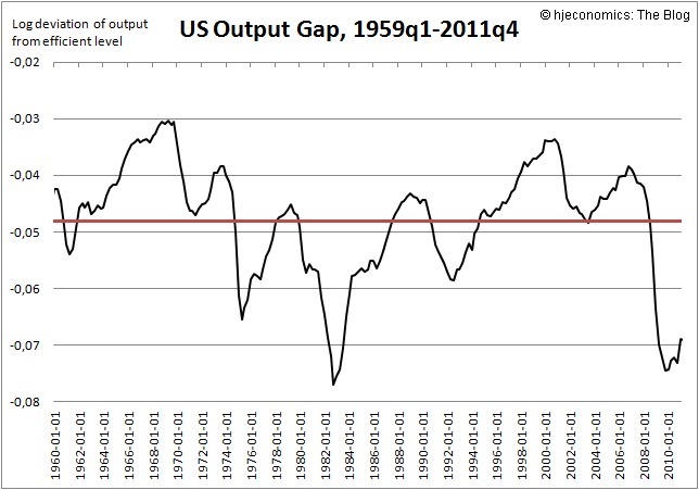
Based on data from the St. Louis FRED database, I compute the theory-based, welfare-relevant output gap for the US, 1959q1-2011q4. This is shown in the figure below, which is essentially a version of Galí’s (2011) Figure 2.1. It is seen that output is always inefficiently low, and that there are substantial fluctuations around an average welfare-relevant output gap of -4,8%. The fluctuations around the average is what I consider relevant for monetary policy, and one sees that currently, output is below this average. So, the output gap is still negative; and of a non-negligible magnitude; by this theoretically-based approach, US output is around 2% below the natural rate of output (and nearly 7% below the efficient level—but this latter number is sensitive to calibration).
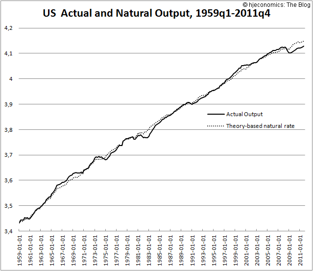
 “Going backwards,” one can use this output gap measure together with actual output data in order to recover the natural rate of output. This is done in the figure below:
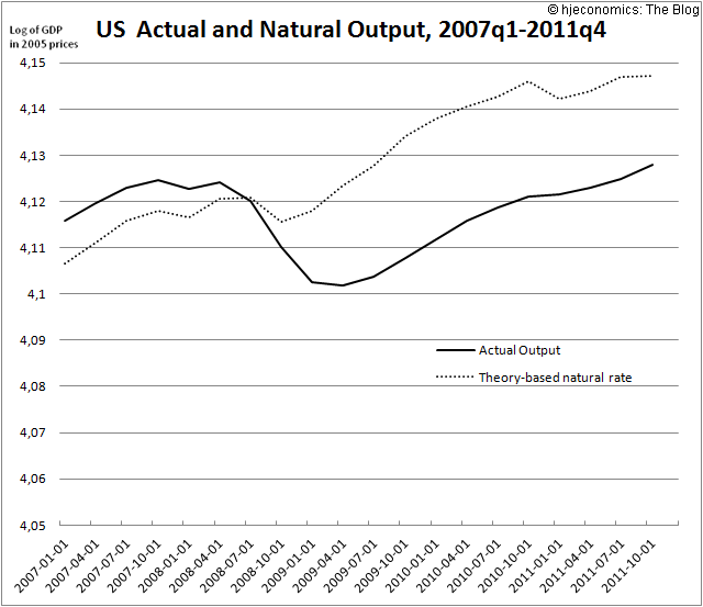
In the last two figures, I take the above figure and zoom in on the periods that John Taylor focuses on, in order to assess the differences between the current recession and the recession in the early 1980s. So I present below the same numbers for the sub periods considered by Taylor: 1981q1-2011q4 and 1981q1-1985q4. Note that the scaling are the same, such that the vertical distance of the figure is 10% of output in both instances (i.e., the distance between the horizontal lines is 1% of output).
It appears correct that the US recovery is slower currently than in the 1980s. However, the recovery only begins in the middle of the considered 5-year span (third quarter of 2009), whereas it starts earlier in the 5-year span in the 1980s considered by Taylor. Moreover, the simple “potential output” figures used by the CBO and Taylor are very smooth, and it is notable that by using the theory-based measure, there was still a negative output gap in the fourth quarter of 1985 of around 0.75% . Only in mid-1987 was the gap closed.
So, while the recovery now indeed seems slower, it did take more time in the 1980s than what the “potential output” figures may suggest. Interestingly, the theory-based natural rate measure grows equally slow in both periods. From 2007-2011 the natural rate of output grew on average at 1,4% annually, while from 1981-1985 the number was 1.2%. In both periods, growth in the natural rate is hampered by periods of no growth.


