The Taylor Plot: A European View

January this year, John Taylor posted a scatterplot on his blog. He plotted quarterly US unemployment against fixed investment as a fraction of GDP for 1990q1-2010q3, and found a very strong negative correlation (jpg ). In contrast, the relationship between government spending and unemployment tended to be positive, albeit not so strong. On the latter finding he notes that “the correlation is not due to any reverse causation from high unemployment to more government purchases”. Overall, he therefore concludes that “Encouraging the creation and expansion of businesses should be the focus on government efforts to reduce unemployment” and further:

“The recent compromise agreement to prevent the increase in tax rates on small businesses and the move to lighten up on the anti-business sentiment coming out of Washington are two steps in the right direction.”

I.e., he reads a causal interpretation into the plot (probably backed by some of the on-going research he mentions in the blog post).

When Greg Mankiw this Tuesday posted the graph on his blog under the heading “A Striking Scatterplot”, the finding got wide attention on the web. Mankiw, the usual admirable cautious academic, remarks that such a plot says nothing about causality, and any interpretation is therefore debatable. I agree wholeheartedly, and also find the correlation impressive. Paul Krugman, on the other hand, has no problems shooting down Taylor’s causal interpretation and adopting the opposite interpretation. He breaks down investment into non-residential and residential components, and argues that it is the recent bust in housing that drives the correlation: Since the housing bust has caused a consumption decline and higher unemployment, all investment is cut back. Any remaining talk is “just politically motivated mythology”. John Taylor responds calmly that the strong correlation is present over the entire period in particular for non-residential investment – a fact, not mythology.

Justin Wolfers then argues that the correlation breaks down if the sample is extended back in time, and labels the Taylor plot an example of “Advocacy Science”. Not surprisingly, Taylor disagrees and presents his case for a longer sample, back to 1960, here. He argues that Wolfers fails to acknowledge that the structural rate of unemployment since 1948 has undergone many but slow changes, which would cause shifts in the scatterplot. I guess this is much akin to the insight that short-term Phillips curves are present in scatterplots even though they over long samples may appear absent because of low-frequency movements in the natural rate (Wolfers can probably still quarrel about the missing period 1948-60 in Taylor’s rebuttal).

Clearly, one cannot say anything firmly about the causal nature of the relationship. But sometimes simple correlations can give you good ideas. So, I looked at Taylor’s plot for the Euro area. For this economic entity, ECB only has quarterly data back from 1995, and I use all that is available as of today. So please no accusations of “advocacy science”; on the other hand, this is not science, just scatterplots. Note that my choices of x and y-axes are arbitrary; they do not indicate subscription to a particular causal interpretation.

The European scatterplot for unemployment and fixed investment looks like this:
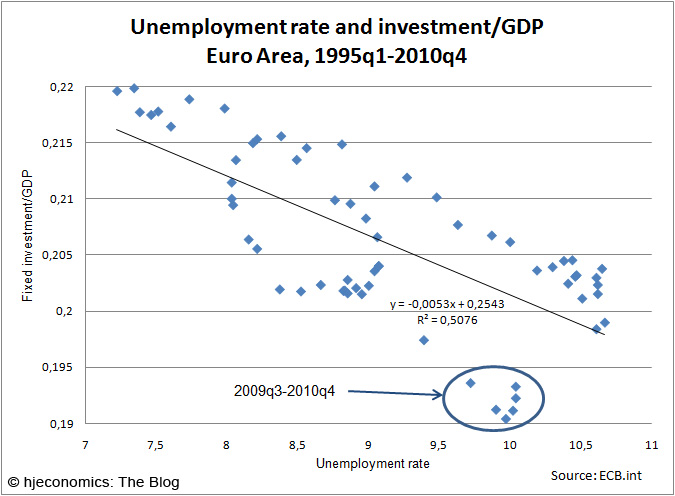
Unemployment rate and Investment/GDP ratio in the Euro Area: ScatterplotThe negative relation is there, but clearly not as impressive as in the Taylor plot. Other GDP components have little correlation with unemployment, except private consumption which shows a positive correlation (probably reflecting a countercyclical average propensity to consume). A time-series representation of the unemployment/investment rate data looks like this:
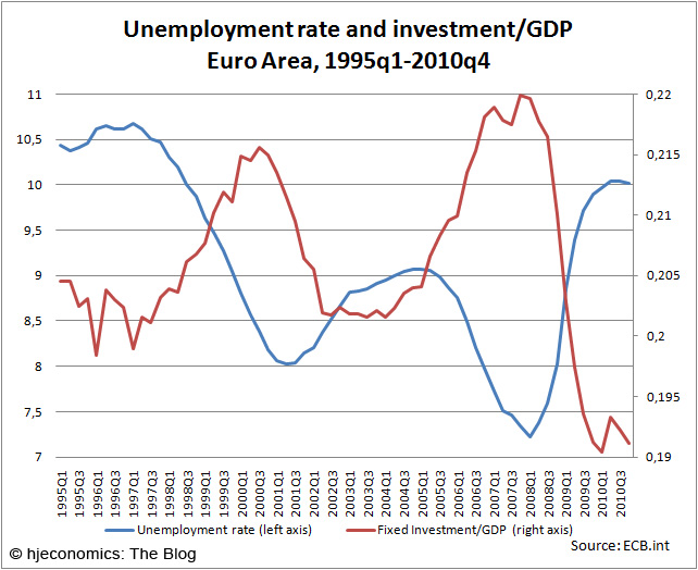
Unemployment and investment/GDP ratio in the Euro area: Time seriesNow, in terms of the correlation between government spending and unemployment also considered by Taylor, Europe looks not at all similar to the US:
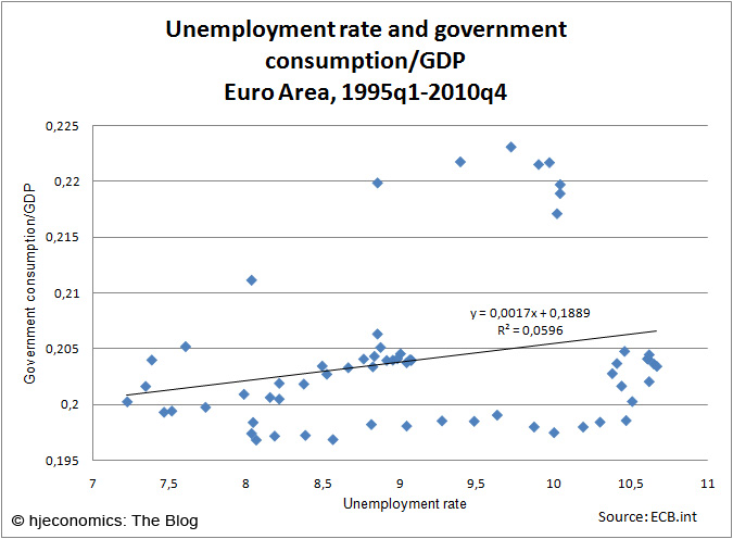
Unemployment and government spending//GDP ratio: ScatterplotUnemployment and government spending are positively correlated as in the US, but very weakly so. I guess it will be relatively hard to build a case for unemployment being created by government spending in the European case.

In terms of the current business cycle downturn, there is an interesting difference between the US and Europe’s unemployment and investment experiences as revealed by the Taylor plot. Note that a group of outliers in the European case are the latest six quarters and that these are below the “fitted” line featuring record-low investment and high, but not historically high, unemployment. In contrast, for the US, Krugman shows in yet another post (focusing now only on non-residential investment), that current times are above a fitted line featuring record-high unemployment and investment around its all-time low (this would also be the case when one looks at total investment).  He therefore concludes that investment in the US is stronger than you would have expected from past behavior given that unemployment causes investment. On that point, Taylor dryly notes that “unemployment is even higher than the high level that would be expected from the low level of business fixed investment”.

We see again that the devil always does lie in the detail (here, he/she is causality). But seen in the gloomy light of the abysmal US performance, Europe almost seems to be deviating from the norm in a good sense. Despite the worst downturn in decades, Europe is not having record-high unemployment, and the record-low investment ratios are still close to a respectable 20%; not bad compared to the current 12% in the US. Some is good for the European economy after all. Funny though, this will make it difficult to formulate easy-selling policy-platform statements, irrespective of your “causal standpoint”. The Krugman-style economist will stumble when explaining, and facing, the fact that unemployment (even though it is not that high) has created abnormal low investment rates. The Taylor-type economist will find difficulties in promoting tax cuts for businesses when explaining that the low investment rates have created surprisingly low unemployment.

Facts are facts, but scatterplots do not tell a story no matter how impressive they are. And the quick, and wildly diverse, policy recommendations drawn from them, should mainly be put forth in political circles and in media. Not by respected academics.

Share
Posted in Economics, Economists, Macroeconomics | Tagged , , , , , , , , | Comments Off on The Taylor Plot: A European View

Taylor Rules on the Taylor Rule

The rule for nominal interest rate setting that John Taylor proposed in his 1993 paper “Discretion versus Policy Rules in Practice“, Carnegie-Rochester Conference Series on Public Policy 39, 195-214, has had an enormous influence in the macroeconomics profession.  It is safe to say that numerous economists, practitioners and academics alike, since that paper have evaluated monetary policymaking using the Taylor rule as some kind of reference point. Empirically, a plethora of papers have estimated coefficients of Taylor-type rules for different countries during different periods. Theoretically, paper after paper on monetary policymaking adopt some form of the Taylor rule as a default specification of monetary policymaking (even undergraduate text books routinely incorporate a Taylor rule as part of the determination of the economy’s AD curve). In practical monetary policymaking, some authorities assess policies relative to what a Taylor rule would have ordered.

Because of its heavy usage in so diverse settings, it has to some gradually become slightly unclear what John Taylor actually meant the rule should represent when he proposed it (this confusion, I am not afraid to admit, has also cursed me). Was it meant as a descriptive or normative concept? In the original paper, he shows, in a now famous Figure 1, how the “example policy rule” tracks the actual US Federal Funds Rate 1987-1992 “remarkable well”. However, he did not choose his rule with the aim of fitting the data. In any case, this may also have contributed to confusion about the proper, and original, interpretation of the rule.

Luckily, there is no need to speculate anymore, as John Taylor himself has now ruled out any potential confusion. On his blog, “Economics One,” he writes in the post “Misunderstanding Prescriptive Versus Descriptive Monetary Policy Rules”:

“. . . the Taylor rule was not meant to be descriptive as I made clear in my original paper. Rather it was very explicitly meant to be prescriptive. I derived it by experimenting with different types of rules in stochastic simulations of different monetary models, including my multi-country model at Stanford, and by studying the results of other people’s simulations. This pinned down the left-hand side variable and the right-hand side variables, and led to simple functional forms and coefficients”

This should clear out any misunderstandings. The following is a prescription for monetary policymaking:

r =  p + 0.5y + 0.5(p-2) + 2,

where r is the nominal (policy-) interest rate, p is the rate of inflation over the past four quarters, y is output’s percentage deviation from trend, and “2” indicates both the (indirect) percentage inflation target and steady-state real interest rate.

In the original paper, Taylor notes that “there is not consensus about the size of the coefficients of policy rules” but labels his rule a “representative policy rule”. That is fine, as there is obviously nothing magic about the number “0.5” (or the now more famous “1.5”. which is the sum of coefficients on the inflation term). Its “derivation” also seems guided by experimentation on some existing models – which exact criteria were used is not spelled out clearly in the paper, which ultimately makes it appear quite judgmental. And a good prescription for policy should be anything but judgmental. Note, by the way, that the precise numbers in the rule do seem important to Taylor today, as he writes:

“You can’t justify QE2 by saying that the interest rate is negative with the prescriptive policy rule I proposed, because the implied rate is not negative, it’s close to 1 percent”

In any case, I am still confused. How can a “representative” interest-rate setting rule that resembles a couple of years of actual policymaking in the US in six years, which is derived by some experimentation, have generality for other time-periods and other countries? Any exercise in optimal interest rate determination in modern DSGE models gives rise to much more complicated rules than the Taylor rule. Nevertheless, the literature often presents arguments like “the Taylor rule performs well”, and sometimes even backs it up by proper welfare measures. However, in my view this merely reflects the fact that such DSGE models feature price rigidities as the overwhelming (monetary policy-relevant) distortion. Thereby, pure inflation stabilization often does a good job, and a Taylor rule will replicate this well with a high coefficient on inflation. So, the rule’s success may reflect simplicity in the models’ policy tradeoffs. This point is clear from some of the work by Stephanie Schmitt-Grohé and Martín Uribe, where they show that the principal role of monetary policy in a common DSGE model is to secure a determinate low-inflation outcome (see, e.g., their 2007 “Optimal Simple And Implementable Monetary and Fiscal Rules,” Journal of Monetary Economics 54, 1702-25).

Now, adherence to rule-based behavior is of course advantageous in face of time-inconsistency problems of monetary policy. However, for a rule to work, it should be credible, i.e., policymakers should stick to it; also when it hurts. On this point the Taylor rule still confuses me. Given that it is a policy prescription, how come that most of the original paper is devoted to discussions of how to deviate from the rule? In the original paper’s concluding remarks it says:

“This paper has endeavored to study the role of policy rules in a world where simple, algebraic formulations of such rules cannot and should not be mechanically followed by policymakers” (from Taylor, 1993, p. 213).

I just don’t get it. A prescriptive rule should not be mechanically followed? But then it is not a complete policy prescription in my view. The terms “rule” and “not mechanically” should simply not appear in the same sentence.

Therefore, despite Taylor’s clarification, I prefer to think about the Taylor rule as a useful descriptive short-hand for policy experiences around the world, as well as a convenient modeling tool to simplify the complications of real-life monetary policymaking.

Share
Posted in Economists, Macroeconomics, Monetary policy | Tagged , , , , , , , , | 1 Comment

Temporary and Permanent Ricardian Confusion: Going Comfortably Numb

Spurred by the heated debates about the need for fiscal stimulus in the US, the issue of Ricardian Equivalence has taken center stage in the economic blogging sphere recently. While it is an impossible task to identify any exact line of events on the net (and possible also irrelevant), this round appears to have been initiated by an article by Justin Yifu Lin (pdf), Chief Economist of the World Bank, who got criticized here by a balanced Antonio Fatás. Fatás notes, among other things, that Lin’s fears that fiscal stimulus could be caught by the “Ricardian trap” (i.e., neutralized by offsetting increased private savings) are unwarranted. While Lin’s endorsement of productive government spending (like public investment) is hard to dispute, it blurs the fact, according to Fatás, that in a depressed economy, spending on perishables can have its own benefits irrespective of the “Ricardian trap”.

That post was then picked up by Nick Rowe and Paul Krugman. Rowe somewhat comes to the rescue of Lin, and has some interesting points about the measurement of government spending, arguing that if spending taking the form of “pure waste,” as considered by Lin, it is equivalent to a transfer payment; i.e., a tax cut. It will therefore have no expansive effects if Ricardian Equivalence holds. Hence, it is indeed important, as Lin argues, that spending is directed towards productive usage. Krugman steps in (step 1 and step 2), and digs out his earlier writings on Ricardian Equivalence, where in one of his many blog posts he writes

“But suppose that the increase in government spending is temporary, not permanent — that it will increase spending by $100 billion per year for only 1 or 2 years, not forever. This clearly implies a lower future tax burden than $100 billion a year forever, and therefore implies a fall in consumer spending of less than $100 billion per year. So the spending program IS expansionary in this case, EVEN IF you have full Ricardian equivalence.

Is that explanation clear enough to get through? Is there anybody out there?”

Yes, I am. And it appears that the thrust of arguments is that a permanent increase in government expenditures is fully crowded out by private consumption rendering it impotent, whereas if the increase is temporary, and counts as GDP, then it is expansive even under Ricardian Equivalence. These claims are just not necessarily correct, as they are based on pure accounting and a simplistic view of private-sector responses to policy changes. Moreover, it generally requires more assumptions to get government spending to be expansive. And most people seem reluctant to mention them. Why, I don’t know. Maybe Fatás has part of the answer when he attributes it to economists’ resistance to be labeled Keynesians; at least I would guess such an explanation fits well for the US (but, luckily, to a lesser extent for Europe I would claim/hope).

So I just want to go through the arguments behind Ricardian Equivalence for the umpteenth time, to make sure that people (and my students) know what it is, and what ramifications it have (or do not have) for the effectiveness and desirability of fiscal policy stabilization. A quick disclaimer from the beginning: I do not believe in Ricardian Equivalence as being a good approximation to reality. Nevertheless, it is clearly formulated theoretical results, which provoke us to think deeper about reality. (I should also note that Fatás last week commented on the debate.)

The Ricardian Equivalence theorem takes as starting point that for a given path of government expenditures it does not matter whether expenditures are financed by deficits or taxes. For the government to satisfy its intertemporal budget constraint (i.e., not running Ponzi games where debt is continuously rolled over and exploding), any change in the path of taxes must be accompanied by an offsetting change in the path of deficits such that the present value of all future deficits and surpluses match the present value of all future government spending (plus the value of initial public debt). So far, this is pure accounting. The big implications come when one combines it with private sector behavior. The path of government net surpluses needed to finance a given path of expenditures is a liability of the private sector. In an idealized world where the private sector is living as long as the government (say, infinity), has access to perfect capital market at the same interest rate as the government, and where taxes are non-distorting, then this liability will not change if government spending does not change. Hence, the strong result: A tax cut has no effect on private sector behavior, as it does not change the present value of the government’s future deficits and surpluses. In words, consumers know that the associated deficit will have to be covered by a tax increase at some point in the future (with interest). They save the tax cut, such that they can be ready to pay the anticipated increases in the future. To repeat, with given government spending the Ricardian Equivalence theorem is clear: Tax and deficit financing is equivalent, and a switch between the two is irrelevant, making consumers in a perfect world be indifferent as well.

When considering changes in the path of government spending, things get much more complicated. Even in the case where Ricardian Equivalence applies (and I assume this throughout as well as I assume that government spending creates GDP), there is now a change in the present value of the government’s total financing needs, and correspondingly a similar change in the liabilities of the private sector. So, from a budget accounting point of view, an increase in government expenditures reduces households’ available life-time resources. The debate is therefore usually focused on whether this reduction is sufficient to fully counteract the increase in government expenditures or not. But then one is inevitably moving away from pure accounting principles and into the realm of private sector behavioral responses towards changes in resources. Hence, it is overtly simplistic to retain a pure accounting approach, and for example state that a permanent increase in government spending leads to a permanent reduction in private consumption of similar size leaving total spending unchanged. This can be consistent with households’ desire to have constant consumption, whereby they indeed each and every period reduce consumption by the same size of the government spending increase. Likewise, it is simplistic to state that a temporary increase in government spending increases total spending. Again it can be consistent with an idea of consumers wanting to keep consumption constant over time: As the drop in the resources is now smaller, their constant per-period consumption falls by less. Hence, total spending will increase (and then drop when the government spending increase is reversed, but that future is rarely spelled out in current times).

The behavioral responses are thus based on an extremely simplistic consumption-is-all-that-matters private sector. Many entirely standard macro models are a tad more complicated than that, and they can therefore easily give the completely opposite results than what, e.g., Krugman is claiming. Think of the situation where households also face a decision about their labor supply. Then, in a classical model (without any dynamics), a permanent increase in government spending increases total spending and production as labor supply goes up (the first-order effect of reduced consumption spending is an increase in the marginal utility of consumption making work more desirable); see. e.g., Michael Woodford, 2011,” Simple Analytics of the Government Expenditures Multiplier”, American Economic Journal: Macroeconomics 3, pp. 2-4. Then think of a Ramsey-Cass-Koopmans model with endogenous capital formation and fixed labor supply. In this model, a temporary increase in government spending instantaneously reduces consumption and investment, leading to falling output and higher real interest rates. Consumption indeed drops immediately by less than the government spending increase, and lesser the shorter policy change, but it starts growing in anticipation of the future reversal of fiscal policy (In the continuous-time version of the model, consumption will remain approximately unchanged if the government spending increase lasts for an infinitesimal length of time – this case appears analogous to Krugman’s two-period, short-run/long-run model, where a short-run spending increase leaves consumption unaltered.) When the increase in government spending is reversed, investment picks up, and output grows back to the initial level (see David Romer, 2006, Advanced Macroeconomics, p. 73). So it all depends on the private sector responses to the policy change. Budget accounting, on which the equivalence theorem is based and satisfied here, is just not doing the job here when government spending changes. So I hope people in the debate would focus more on specifying what transmission mechanism they have in mind instead of insisting on this merely being a matter of permanent versus temporary changes in government spending. It is clearly not.

The models used to exemplify the confusion are both flex-price supply-side models. Obviously, they are rigged against providing a rationale for expansive fiscal policies against unemployment problems, but in newer sticky-price models, government spending is usually expansive also under Ricardian Equivalence (for the mundane reason that output is demand determined). Actually, most New-Keynesians models focus on Ricardian Equivalence for simplicity. And temporary and permanent fiscal expansions can have positive output effects in these models (the models, however, have some problems replicating that private consumption often increases with government spending). And I would imagine that most economists favoring demand management policies to have some Keynesian sympathies (despite that they may not admit it as Antonio Fatás wrote). Read Pierpaolo Benigno, 2009, New-Keynesian Economics: An AS-AD View, NBER Working Paper, No. 14824 for a simple and clear exposition, which also covers distortionary taxes. Note however, that the flex-price scenarios are not just theoretical playgrounds that silly mathematical economists like to fumble around with. They are the ones policy should aim at replicating as close as possible. One of the main contributions of the New-Keynesian literature is indeed the focus on designing policy to be stabilizing welfare-relevant gaps between, e.g., output and its natural (flex-price) level.

It is therefore very important, as always in economic debates, that people are transparent about what their essential assumptions are. Otherwise things will end in a shouting contest where participants are being, or faking to be, completely numb. It may be comfortable to rest unaffected with one’s old arguments, but economics is not about being right. It is about getting smarter. So, when Paul Krugman ends by crying out “Is There Anybody Out There?”, I feel the urge to extend my “Yes” with:

“Relax
I need some information first
Just the basic facts
Can you show me where it hurts?”

From “Comfortably Numb”, music by David Gilmore/Roger Waters, lyrics by Roger Waters. © 1979 Pink Floyd Music Pubs. Ltd. All rights reserved.

Share
Posted in Economists, Macroeconomics | Tagged , , , , , , , , , , , | 2 Comments

The Fed and the ECB: “Spurious Bedfellows”

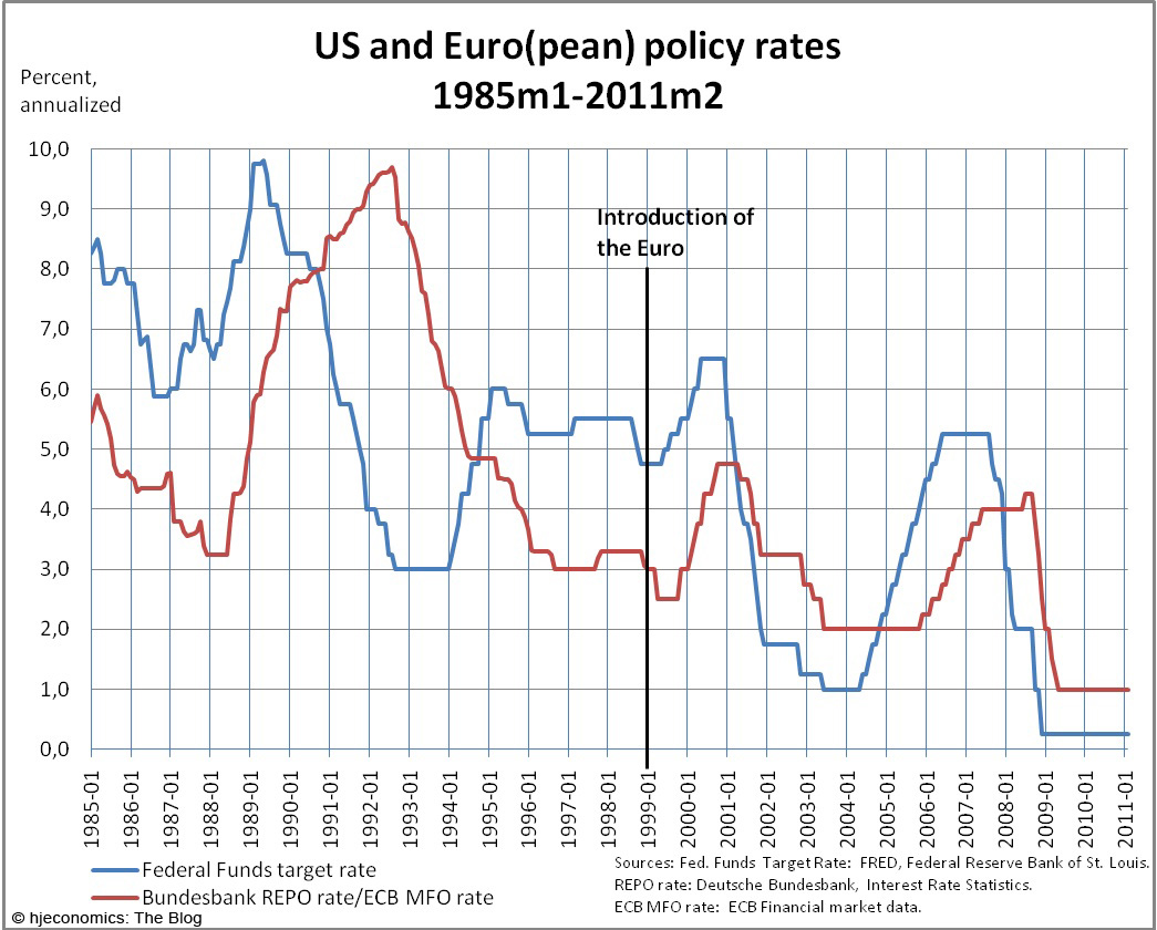
Some days ago, I wrote about an interesting post by Gavin Davies on his Financial Times blog, where he argued that European monetary policy, through the actions of the German Bundesbank and now the European Central Bank, follows the US Federal Reserve’s interest rate decisions with some delay. An observation leading him to label the FED and ECB “strange bedfellows”. The data behind the argument is seen in the following figure:

US and Euro(pean) monetary policy 1985-2011

The Federal Reserve’s policy intentions are throughout the period measured by the target value for the Federal Funds Rate (formally, this time series is discontinued as of December 2008, and I show the upper value of the 0-0.25% target range of the Fed for subsequent periods). European monetary policy is measured by the Bundesbank’s Repo rate up until the end of 1998. From 1999 and onwards, the rate for main refinancing operations set by the European Central Bank is used. Indeed, by eyeballing the figure, it appears that Europe is following the US. My own eyeballing led me to conjecture that much of the thrust behind the argument came from the events in the early 1990s where the Fed’s rate cuts in 1990-93 were followed by the German cuts in 1992-95. Hence, the ECB may not be much of a follower.

Well, eyeballing is never a good idea when it comes to data. We have statistical methods for making inference, and my eyeballing was indeed way off. I have measured the cross correlation for the policy rates for the entire sample, as well as for the subsample involving the existence of the European Monetary Union.

Fed Funds Rate and European monetary policy; cross correlation 1985-2011

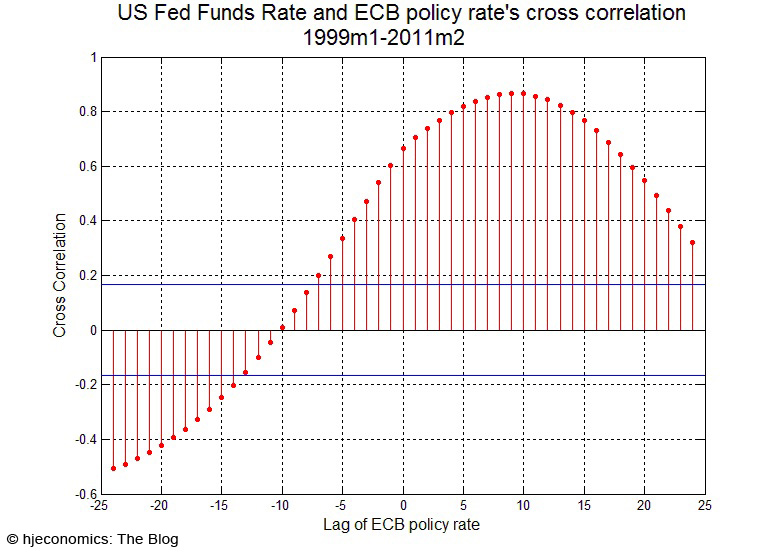
Fed Funds Rate and ECB monetary policy; cross correlation 1999-2011

From these cross correlations one sees that the highest correlation actually arises in the ECB-only subsample. Indeed, as Gavin Davies reported, at lag 10 the correlation coefficient is over 0.8; a value not reached over the entire sample. In either sample, however, the Fed’s actions are indeed leading the ECB’s. However, these cross correlation functions also reveal a highly disturbing feature.

Cross correlation functions displaying the oscillatory patterns seen in these figures are known to occur when data are highly persistent and trended. And in fact, both policy-rate series are highly persistent and both are trending downwards. These properties lead to the well-known phenomenon of spurious correlation. One cannot reject that the series have a unit root, but leaving that controversial issue aside, it has been known for long time that series with ARMA (Auto Regressive Moving Average) properties may exhibit significant and oscillatory cross correlation functions even though the series are statistically independent. I.e., the measured correlation is spurious. An early “pre-unit-root literature” reference is Awe, O., 1964, Errors in correlation between time series, Journal of Atmospheric and Terrestrial Physics 26, 1239-1255.

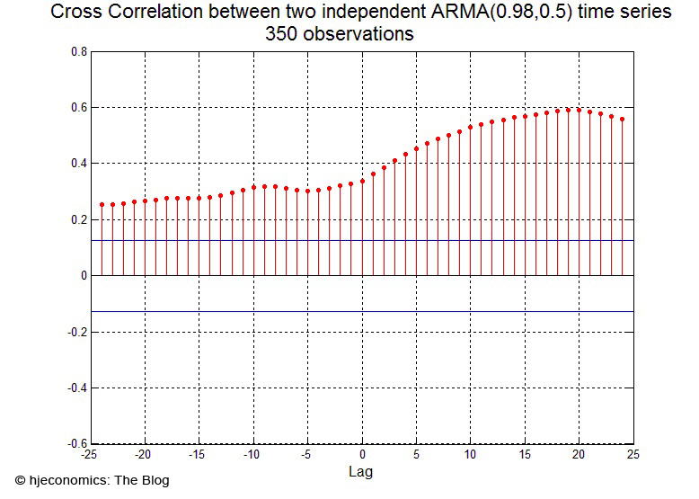
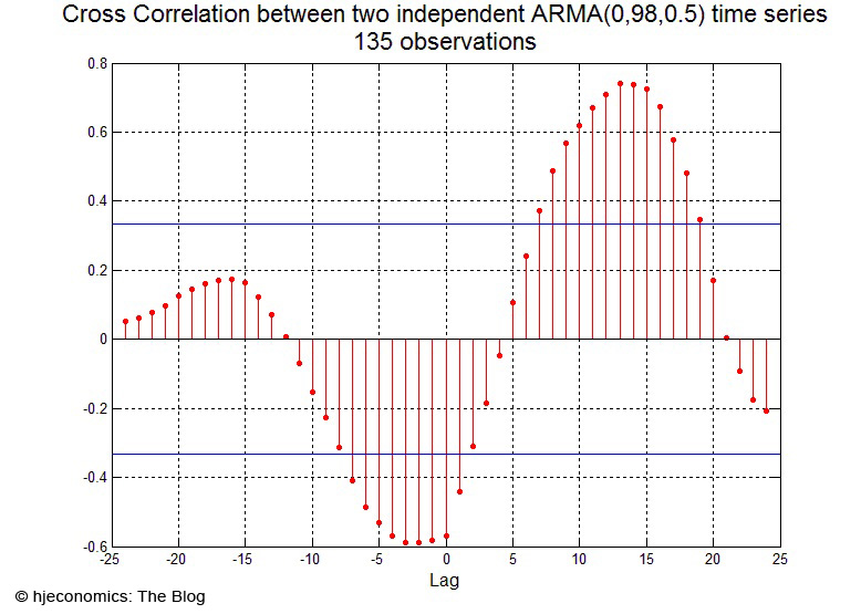
As means of illustration, I show figures for the cross correlation functions between two statistically independent ARMA processes for a long and shorter sample (mimicking the Fed/Europe and FED/ECB sample lengths, respectively):

Spurious cross correlation between two independent ARMA time series

Spurious cross correlation between two independent ARMA time series (again)

As evident, even though the time series have no relation whatsoever by construction, their persistence accounts for a spurious cross correlations quite similar to the one found in the monetary policy data.

So, my eyeballing was not on the spot. A formal statistical examination, however, reveals that there is not basis for placing the Fed and the ECB in the same bed. At least not from looking at simple cross correlations extracted from the raw data.

Share
Posted in Economists, Macroeconomics, Monetary policy | Tagged , , , , , | Comments Off on The Fed and the ECB: “Spurious Bedfellows”

Freakonomics: The Movie Review

In 2005, economist Steven D. Levitt and journalist Stephen J. Dubner published the book Freakonomics, which in a remarkable lucid manner demonstrated the power of economic thinking to a wide audience. Focusing on the importance of incentives, the authors guided the reader through a range of Levitt’s research on diverse topics as cheating in sumo wrestling, price setting in real estate markets, living habits of drug dealers, the potential importance of naming conventions for children’s future, and the probably most controversial topic (in practically any aspect): the potential impact of legalized abortion on crime rates. The book provided new and provocative insights into what economists can do with their toolboxes, and I must admit that I have given it as a gift many times to make people understand that economics is not just about more mundane things as whether an increase in the inflation rate of 0.1 percentage points is a sign of coming disasters. And many are the times I have gotten in trouble when explaining that the fall in the crime rate in the 1990s in the US could be due to legalization of abortion in the 1970s in the sense that a lot of criminals as a consequence were simply not born. People have a hard time distinguishing the narrative from the non-existent agenda behind the research, and some have concluded that the authors must be racists, Nazis or worse, and that I more or less much be the same, when I find such research of interest. In other words, I like the book a lot.

As is the case of many bestsellers, the book has now been turned into a movie. Thereby, it must be among the very first economics books ever getting that treatment. When I say “now”, I am being slightly misleading, but the 2010 documentary did not get theatrical distribution in Europe, so I had to wait for the DVD release. Now I have it, and have seen it. I was worried beforehand, as successful books rarely turn into good movies. There are exceptions, of course (The Godfather and The Name of the Rose come to mind), but often good adaptations come from lesser known books (think Psycho). Judged by the credits of the movie, however, I couldn’t help have my hopes up: Seth Gordon, who directs a number of smaller segments of the film, has assembled a group of high-profile documentary filmmakers to each make a longer mini-documentary on one particular subject from the Freakonomics universe.

Gordon’s segments are mainly shots of Levitt and Dubner explaining and discussing various subjects, spiced up with cartoonish graphics to get the points through. Some segments are well crafted, but some appear not sufficiently complete. In contrast with the book, e.g., one does not learn what special pattern Levitt searched for, and found, to discover that teachers deliberately altered student’s test scores to the better. We just see a bunch of flying numbers, which gradually form a number of identical sequences that are then eventually aligned on top of each other. Wow! And on to the next subject. As an example of how correlations have nothing to do with causality, Levitt and Dubner tell the story about how polio in the 1950s was being suspected to be related to ice-cream consumption. The reason being that polio mostly broke out during the summer. Well, what did cause polio to break out mostly during the summers, now that it obviously wasn’t ice cream consumption? To the viewer, a hint to the actual solution would be a nice closure. In between these small segments are the four mini-documentaries that constitute the main parts of the movie.

“A Roshanda by Any Other Name” is directed by Morgan Spurlock (Oscar nominee for Super Size Me in 2004), and tells the story about how names may affect children’s success in life. It is done in a rather conventional news-segment style with emphasis on interviews with people on the streets and statements by a few experts on names. We are presented for evidence that names convey ethnicity, which then can affect job opportunities, but the segment more or less fades out with smiling faces assuring the viewer that it doesn’t really matter what you name your kid. Why bother then? The segment “Pure Corruption” is directed by Alex Gibney (Oscar winner for Taxi to the Dark Side from 2007), and is by far the best part of the movie. It could easily have been developed into an intriguing full-length documentary in itself. Its point of departure is the detection of Yaochō (match fixing) in professional sumo wrestling. The way the tournaments are set up, creates matches where the outcome is pivotal for one wrestler and almost irrelevant for the other; in accordance with incentives, the wrestler with most to win actually wins most of the times, even though he subsequently may lose several times to the same opponent. Evidently, this smells of cheating. The segment goes much deeper than this, however, and focuses on the special codes of honor prevailing in the hierarchy of sumo wrestling. It is great filmmaking with a clear narrative presenting fascinating accounts on tragic and controversial events within this special sport. In the process, it wanders away from the subject of economics, and maybe therefore some weak analogies between corrupt leading figures in the sport and corrupt financial tycoons (Bernie Madoff and others), who are held responsible for the recent financial crisis, are thrown in at the end. A disappointing and abrupt finish to a fascinating view into a different world.

“It’s not Always a Wonderful Life” directed by Eugene Jarecki (who made the critically acclaimed Why We Fight in 2005), is the segment that explains the story about abortion and crime rates. It is told by a voice-over narrator, and breaks the continuity of the overall movie by spending time introducing Levitt as if we didn’t already knew him. Maybe I getting overtly sensitive, but I found the exaggerated (ab)use of clips from Frank Capra’s 1946 masterpiece It’s A Wonderful Life quite disturbing. In that movie, for those few who do not know it, James Stewart’s suicidal character, George, is by divine intervention given the chance to experience life in case he wasn’t born. The experience cures his depression and makes him want to live again. Hence the title of the movie. The name for the segment is of course a nod to Capra, but it has the unfortunate implication of reversing the morale of the original movie: Apparently it can be better not to be born after all. Thereby, it, in my eyes, takes a stand on abortion, which it otherwise does everything so as to avoid. It ultimately appears clumsy at best.

The last major segment, “Can a Ninth Grader Be Bribed to Succeed?” is directed by Heidi Ewing and Rachel Grady (Oscar nominees for their 2006 Jesus Camp). It follows an experiment run by Levitt and others (not in the original book) in which they test whether monetary incentives can induce better studying habits among ninth grade students. Students are through the year awarded $50 whenever their grades improve appropriately, and they become eligible for participating in a lottery for a $500 equivalent prize (involving driving around in a huge limo). To make the story of human interest, we closely follow two students with initial low grades, and their various ways of trying to improve. From that point on it turns into what looks like a conventional reality-TV show: Who will win? It is semi-dreadful to watch, and one of our young friends not only improves his grades to earn him $50, but he also wins the full $500 prize (the other one did not respond to incentives). This must have been a very expensive mini-documentary to shoot, as the directors surely have followed the everyday life of all students participating in the experiment, such that they could be certain to have extensive footage of whoever would win in the end. Alternatively, the whole thing is just bogus, as are the kind of cheap TV shows it mimics so well. At the end, Levitt and his fellow researchers are seen discussing the preliminary results of the experiment, and apparently they are disappointed with the measured incentive effects. We then hear Levitt off screen contemplating a redesign of the experiment, addressing new questions, and concluding that it will be fun. Yes, fun. Well, economics is fun and interesting at the same time. I will definitely not dispute that, and I applaud any attempt to disseminate that fact to a wider audience. But the segment and the whole movie, being comprised of such diverse styles of filmmaking, give the impression of Freakonomics just being about having aimless fun. Fun for the sake of fun (Levitt and Dubner are indeed laughing most of the time when they are on camera). The movie misses out on giving the viewer a sense of the importance of economic thinking, which is just as crucial as the fun. A job the book did so very well.

So overall, and I hate to say it, the movie is a disappointment. Maybe I had too high hopes, or maybe I couldn’t be sufficiently surprised by most of the stories since I have read the book. I don’t know, but ex post I would have preferred reading the book again instead. And Alex Gibney should clearly have done an independent documentary on sumo wrestling.

Freakonomics at IMDb

Share
Posted in Economics, Movies | Tagged , , , , , , , , | Comments Off on Freakonomics: The Movie Review

Brady replaces Woods in Principles

From N. Gregory Mankiw’s description of the new material in the new edition of his “Principles of Economics“:

“Chapter 3
Tiger Woods changed to Tom Brady in in-text example.”

This must be the final blow to Tiger Woods’ status as a respectable sports icon.

Share
Posted in Macroeconomics | Tagged | Comments Off on Brady replaces Woods in Principles

Gavin Davies on the Fed and the ECB

Gavin Davies has an interesting post on his Financial Times blog. It is entitled “Strange bedfellows – the Fed and the ECB” and it discusses the co-movements between the Federal funds rate and the Deutschmark/Euro policy rate since 1987. There seems to be a leader-follower pattern, in the sense that Europe has followed the Fed with a 6-12 month lag. Davies concludes that this “is one of the most well established rules in the analysis of monetary policy making“.

This is perhaps a somewhat strong statement, and I would, based on visual inspection (upon which one should be VERY careful), conjecture that most of this correlation is driven by the Fed’s rate cuts in 1990-93 along with the German cuts 1992-95. Hence, the leader-follower pattern may actually not be as evident for the actual Fed/ECB relationship. In any case, as Davies notes, the scene may soon be set for a divergence of any possible prior Fed leadership as the ECB is soon believed to raise rates while the Fed appears set upon keeping rates unchanged for a while.

(I also managed to post a minor comment to Davies’ post pertaining to inflation targeting and Taylor rules.)

Share
Posted in Economics, Macroeconomics, Monetary policy | Tagged , , , , | Comments Off on Gavin Davies on the Fed and the ECB

ECB, SMP (II): Direct vs. secondary purchases

In my recent post on the ECB’s Securities Market Programme (SMP), I noted that the programme was in violation of the Treaty of the European Union. I based this on Article 21.1, which states:

“. . . overdrafts or any other type of credit facility with the ECB or with the national central banks in favour of Union institutions, bodies, offices or agencies, central governments, regional, local or other public authorities, other bodies governed by public law, or public undertakings of Member States shall be prohibited, as shall the purchase directly from them by the ECB or national central banks of debt instruments.”
– Article 21.1 of “ON THE STATUTE OF THE COURT OF JUSTICE OF THE EUROPEAN UNION”, in “Treaty on European Union and Treaty on the Functioning of the European Union“, 2008.

I also mentioned that ECB Governor Jean-Claude Trichet in this interview stated that the programme is not violating the letters of Treaty, and that I therefore obviously did not understand article 21.

I indeed did not. The key behind my misjudgment is the word “direct” in the Treaty. I failed to understand that this means that “indirect” purchases of government debt are just fine. And “indirect” purchases are indeed what the ECB is carrying out. They explicitly operate on the secondary market for government bonds; i.e., they purchase at financial institutions.

So Trichet is correct. The ECB is not violating the letters of the Treaty by the SMP. I can’t, however, help wondering whether this was the intention of the treaty. It is difficult to imagine the founding fathers/mothers to have contemplated: “Let us forbid the future EU central bank to bail out any EU government in fiscal distress”. “Oh well, let us not, let us just make sure that it does so through financial intermediaries”. (To emphasize, the ECB is currently not monetizing public debt, as they withdraw the liquidity from bond purchases on an ongoing basis.)

In June 2010, a month after the initiation of the SMP, Trichet also said, when asked about certain European countries potentially defaulting on their debts: “We won’t allow that to happen“.

Share
Posted in Economics, Macroeconomics, Monetary policy | Tagged , , | Comments Off on ECB, SMP (II): Direct vs. secondary purchases